Visualising Algorithms with Python

Posted on Tue 29 January 2019 in python

One of the themes for this term is algorithm optimisation, so I've been looking over industry standard sort and search algorithms, ever trying to minimise the 'Big O'. A classmate shared these sort visualisations by morolin, which really help to visualise the differences in efficiency between the algorithms. While these visualisations were created in Golang, they have since been translated in to Python by Kirk Kaiser.

Let's face it, writing code to sort a list isn't particularly interesting, so I wanted to see if I could impliment and visualise my own sort algorithm(s). The next step of course, was to see if similar visualisations could be created to demonstrate search algorithms..

Taking the Red Pill¶

The initial set-up is largely based on Kirk's blog (the key take home message is the key to creating these visualisations is to define your colour template in HSV rather than RGB, as this creates a single attribute on which you can sort). First create a sorted matrix, and then apply a shuffle to randomise the order. In order to visualise the matrix, a conversion from HSV to RGB is required.

In [3]:

%matplotlib inline

from skimage import color, img_as_ubyte
import imageio
import numpy as np
import matplotlib.pyplot as plt

img = np.zeros((100, 100, 3), dtype='float64')

for i in range(img.shape[0]):
    scalar = img.shape[0] * 1.3  # modify the range of colours to trim white from the colour scale
    img[:,i,:] = (i+(scalar-img.shape[1]))/ scalar, (i+(scalar-img.shape[1]))/ scalar, 1.0
    
sort_rgb = color.convert_colorspace(img, 'HSV', 'RGB')

for i in range(img.shape[0]):
    np.random.shuffle(img[i,:,:])
    
shuffle_rgb = color.convert_colorspace(img, 'HSV', 'RGB')

pad = np.ones((img.shape[0], int(img.shape[1]/10), 3), dtype='float64')
plt.figure(figsize=(9,4))
plt.imshow(np.hstack((sort_rgb, pad, shuffle_rgb)))
plt.axis('off')

Out[3]:

(-0.5, 209.5, 99.5, -0.5)

Bubble Sort¶

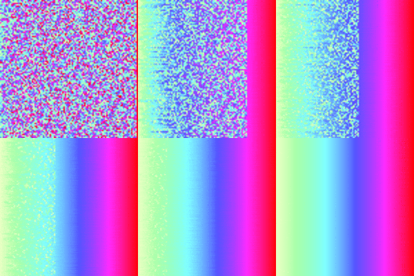
Here's my attempt at a bubble sort implimentation. An additional dimension has been added to the matrix to represent time (one sequence), which will allow us to 'flick' through the data to create a visualisation in the next step. A couple of frames are plotted from different time intervals to make sure that the implimentation is performing as desired.

In [4]:

def bubbleSort(np_matrix):
    seq = np.zeros((np_matrix.shape[0], np_matrix.shape[0], np_matrix.shape[1], np_matrix.shape[2]))
    for i in range(np_matrix.shape[0]):
        for j in range(np_matrix.shape[1]):
            for k in range(0, np_matrix.shape[0]-i-1):
                if np_matrix[j][k][0] > np_matrix[j][k+1][0]:
                    np_matrix[j][k][0], np_matrix[j][k+1][0] = np_matrix[j][k+1][0], np_matrix[j][k][0]
                    np_matrix[j][k][1], np_matrix[j][k+1][1] = np_matrix[j][k+1][1], np_matrix[j][k][1]
                    np_matrix[j][k][2], np_matrix[j][k+1][2] = np_matrix[j][k+1][2], np_matrix[j][k][2]
        seq[i] = np_matrix
    return seq

bubble_sort = bubbleSort(img)

bubble_s39_rgb = color.convert_colorspace(bubble_sort[39], 'HSV', 'RGB')
bubble_s69_rgb = color.convert_colorspace(bubble_sort[69], 'HSV', 'RGB')

plt.figure(figsize=(14,4))
plt.imshow(np.hstack((shuffle_rgb, pad, bubble_s39_rgb, pad, bubble_s69_rgb)))
plt.axis('off')

Out[4]:

(-0.5, 319.5, 99.5, -0.5)

Visualisation¶

The final step is convert each time dimension in the matrix to a frame within our visualisation. I've commented this out from the Jupyter noteback, and the outputs will be referenced directly later on.

In [5]:

#frames = []
#for i in range (0, img.shape[0]):
#    frames.append(img_as_ubyte(color.convert_colorspace(bubble_sort[i], 'HSV', 'RGB')))
#imageio.mimsave('bubble_sort_anim.gif', frames)

Linear Search¶

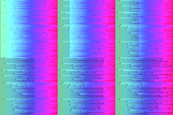
Following the same process, we'll now impliment a visualisation for a linear search. The input data varies slightly in that matrix is now sorted, but with a non-regular increment. A key is randomly selected for each row, and shown by a dark grey pixel within the plot. As the search algorithm scans through the data, it's progress is demonstrated by dropping the pixel value (hsV). Once the key is found, the pixel turns black and the search is terminated for the specific row.

In [6]:

import random as rand
img2 = np.zeros(img.shape, dtype='float64')

rand.seed(1)
max = 1 / img2.shape[1]
key_idx = []

for i in range(img2.shape[0]):
    start = 0.4
    for j in range(img2.shape[1]):
        value = start + rand.random()*max
        img2[i,j,:] = value, value, 1.0
        start = value
    key = rand.randint(0, img2.shape[0]-1)
    img2[i,key,2] = 0.5  # Set random key (value) to black, maining ordered no. (hue)
    key_idx.append(img2[i,key,0])

ordered_rgb = color.convert_colorspace(img2, 'HSV', 'RGB')
plt.figure(figsize=(4,4))
plt.imshow(ordered_rgb)
plt.axis('off')

Out[6]:

(-0.5, 99.5, 99.5, -0.5)

In [7]:

def linearSearch(np_matrix, key):
    seq = np.zeros((np_matrix.shape[0], np_matrix.shape[0], np_matrix.shape[1], np_matrix.shape[2]))
    solve = np.zeros(np_matrix.shape[0])
    for i in range(np_matrix.shape[0]):
        for j in range(np_matrix.shape[0]):
            if solve[j] == 0:
                for k in range(i, i+1):
                    if np_matrix[j][k][0] == key_idx[j]:
                        np_matrix[j][k][2] = 0.0
                        solve[j] = 1
                    else:
                        np_matrix[j][k][2] = 0.8
        seq[i] = np_matrix
    return seq

linear_search = linearSearch(img2, key_idx)

In [8]:

#frames = []
#for i in range (0, img.shape[0]):
#    frames.append(img_as_ubyte(color.convert_colorspace(linear_search[i], 'HSV', 'RGB')))
#imageio.mimsave('linear_search_anim.gif', frames)

Sort and Search Algorithms Visualised in Python¶

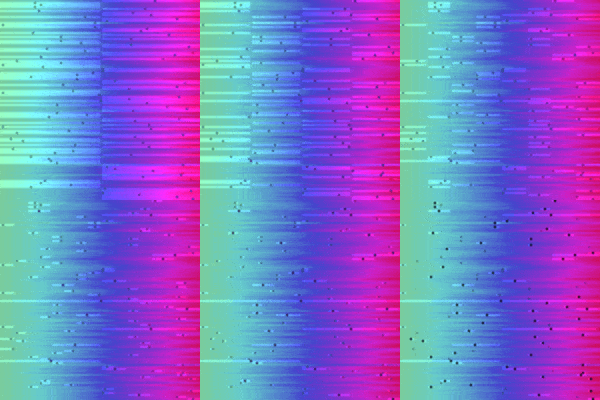
So here are the visualisations on a common time-scale:

Bubble Sort	Linear Search	Binary Search

I was suprised just how efficient the binary search was compared to the linear search, it certainly has the 'Big O' factor.

It would nice to see how these can be made larger without losing resolution in the future, and perhaps try out a few more algorithms!